Solver Design#
Many users of MatchMove software find that by understanding how the underlying processes of the software work they are able to obtain better results by utilising the software as it’s intended to work.
This document tries to answer that question;
How does the MM Solver work?
How does the solver work?#
The solver inside MM Solver is an optimisation solver. The solver attempts to optimise the measured error with various unknown parameter values. The solver’s purpose is to find the parameter values which minimise the measured error.
The process of applying an optimisation solver to 3D perspective cameras, 2D points and 3D points is called Bundle Adjustment (BA). BA is traditionally the last step of MatchMove and Photogrammetry solvers where the parameters of 3D points (Bundles) and cameras are solved to produce a 3D Scene with the least possible error.
Attributes#
In the MM Solver, we refer to unknown parameters as Attributes. Attributes are the Maya attributes that are allowed to be modified inside the solver. Maya attributes that are not added into the solver will still be used, but cannot be modified.
The Attributes modified in the MM Solver may be any attribute in Maya. Likewise the attributes may be in any space required, for example; object-space, world-space or normal/vertex space. The only requirement is that the Attribute modifies the Bundle position (see below for detail on Bundles). Bundle positions may be modified indirectly using hierarchies or rigs of Maya transform nodes. The true power of the solver comes from the evaluation environment, Maya, and the node networks/hierarchies created by the MatchMove artist.
Like Maya attributes, MM Solver Attributes can also change over-time using an animated curve, or just have a single static value, or they can be be locked. Locked attributes cannot be modified by Maya and therefore cannot be modified in the solver either. Due to underlying solving algorithm only floating-point attribute values can be solved. Commonly solved Attributes are 3D translate and rotate axes.
Markers and Bundles#
Markers and Bundles are used to compute the measured error inside the solver. The word Marker is used to describe a 2D point on an image plane, and Bundle to describe the 3D Point.
Markers have had different names in various MatchMove software applications; Track, feature, 2D point, etc. For the purposes of MM Solver name Marker is used for the tracking markers placed on the set of a film production. Bundles are named as such because they represent a bundle of light forming on the imaging sensor.
Markers and Bundles are linked together. The Marker is the representation of the Bundle from a camera’s point of view. There may be multiple 2D Marker representations of the same 3D Bundle.
Having known 2D Markers of a 3D Bundle looking through a known perspective Camera we can calculate a 3D Bundle position by moving the Bundle until the difference between all Markers and Bundles is zero when looking through each perspective Camera. Another way to say this is that the measured error is the distance between the screen-space re-projected 3D Bundles with the linked 2D Markers.
Solving#
Once the solver has Attributes, Cameras and Markers and linked Bundles, the solver can start a solve.
The solver may only start if some conditions are met. One important condition is the number of Attributes verses the number of Markers or specifically:
The number of measured errors must be equal to or greater than the number of Attribute values you’re solving.
All 3D MatchMove software has this limitation, MM Solver is no different. There is a minimum number of Markers required to solve for a 3D Camera that can move in 6 degrees of freedom (6 DOF: translate X, Y and Z, rotate X, Y and Z). For MM Solver this number is a minimum of 3 Markers. 3 Markers are required to solve for 6 attributes.
Since each Marker measures 2 errors (X and Y distance to Bundle), the marker can solve for 2 attributes. For example, 1 Marker can be used to solve a Camera transform rotate X and Y (tilt and pan) attributes.
When the user gives a Marker as input for MM Solver, the position is assumed to be correct. Some 3D MatchMove software applications use many 2D Markers and filter out the badly tracked points (the outliers), MM Solver does not work like this. Badly tracked Markers will affect the solve badly.
This solver is an optimiser and it needs to be provided with an approximation of input attribute values, or in other words; we need to animate the camera(s), and place the bundles in the roughly correct positions. You don’t need to do the job of the solver, which is to make the Cameras and Bundles match perfectly, but you are required to at least have Bundles positioned inside the FOV of the camera, and an approximate animation of the camera if you’re solving the camera parameters.
The approximate Camera and Bundle positions is why the MM Solver is so different from traditional MatchMove solutions, especially Auto-Tracking 3D MatchMove software; there is no one-click solution. But this can be a good thing!
Remember the solver is an optimiser and it re-uses the input parameters and refines them rather than re-starting the solve from scratch. This type of solver enables customised, layered solving. For example, you may solve for a small number of individual Attributes with specific sets of Markers and Bundles, or you could use it in a similar way to other 3D MatchMove software where all parameters are added into the solver.
Due to the inherent refinement nature of the solver, a general process for solving will be:
Add Cameras, Bundles and Markers.
Track 2D Markers.
Place Cameras and Bundles into approximate positions.
Set up movement constraints or node hierarchies for Cameras and / or Bundles.
Solve for Attribute values.
Repeat steps 2-5 until desired result is achieved.
Solving Process#
Each time you execute a solve, the solver goes though a number of steps to perform the optimisation and reduce the error.
This is an overview of the solver’s process:
Initialises input data.
Solve.
Measure Initial Error.
Set all the initial Attribute values.
Measure the initial re-projection error.
Discover how each Attribute changes the measured error.
Iterate.
Based on the discovered value/error changes predict better Attribute values.
Set all Attribute values with the predicted Attribute values.
Measure the re-projection error.
Check if the error is low enough, if so stop solving, otherwise repeat the iteration.
Get solver information.
Set attributes values as calculated.
Measure Final Error.
Get number of iterations.
Return Solver information to the user.
The slowest step of the solving process is step 2 as it may be executed hundreds or thousands of times, depending on the number of Attributes and Markers that are in the solve.
Time - Static and Animated Attributes#
Up until now we’ve been concerned with solving a single frame in time. Now we need to extend that into multiple frames. In the MM Solver there are animated Attributes that change per-frame and static Attributes that only have one value. Using static Attributes complicates the solving process.
If we are to solve only per-frame that would mean Attribute values from one frame would never affect another frame and therefore we can safely loop over each frame and solve each frame individually. When including static Attributes, the static Attributes affect all frames in the solve.
Consider a simple example; 1 animated Attribute and 1 static Attribute, solving on three frames, frame 1, 2 and 3. The animated attribute contains 3 values, an individual value for each frame, and so each value affects the measured error on each frame. But the static Attribute contains only one value, not one for each frame, and therefore the single value affects the measured error on all frames. To solve for the minimum possible measured error for all values it is necessary to consider all 4 values together (3 animated values, 1 static value), and all combinations of the values. Solving for 4 values rather than 3 values doesn’t sound like it would take much longer to compute, but in fact it takes 3 times longer (3 * 3); this problem is squared each time a static value is added. The more static values added to the solve increases the number of possible combinations and increases the number of solver evaluations required for a low measured error. Solving Animated and Static values as described is a Brute Force approach, but other strategies may be used.
Attribute Value Evaluation at Different Times#
This topic is unrelated to the actual solver engine in mmSolver, but documents an interesting implementation detail when correctly evaluating values at different times in Autodesk Maya. From mmSolver v0.3.10 the new mmSolver command flag ‘timeEvalMode’ was introduced to tell Maya how to evaluate values at different times.
There are two different methods to query a value at a specific time, 1) tell the Maya DG network to evaluate a value at a time (using a “DG Context”), or 2) change the Maya scene’s current time, then query the current value.
Tests have shown that the two different methods do not always evaluate the same way and can lead to an incorrect solve if set incorrectly. For simple scenes, method 1 works most of the time, however when using character rigs or complex node networks and evaluating on a single frame, then method 2 is needed to solve correctly.
- Use method 1 when you are solving multiple frames at once, and you
are using the Maya GUI (not Maya Batch or ‘mayapy’).
Use method 2 when you are evaluting a single frame, or when you are not using the Maya GUI such as with Maya Batch or ‘mayapy’.
These different methods do not need to be set manually if you are using the mmSolver Solver UI or the mmSolver API. If you are calling the ‘mmSolver’ command directly, then ‘timeEvalMode’ is important to set.
Attribute Details#
Attribute Details are properties of an Attribute. Attribute Details are used to add constraints such as value limits.
In mmSolver, there are 2 details per-attribute; minimum and maximum. See below for more details on how each property works.
Minimum and Maximum Limits#
Minimum and maximum limits will force mmSolver to solve an attribute with-in specific values. Attribute min/max limits apply to both static and animated attributes. If a mnimium or maximum value is not set, the limit is removed and any value may be used.
mmSolver allows a combination of minimum and maximum limits. The combinations are; minimum only, maximum only, both minimum and maximum, no to limits at all.
Although min and max limits may appear to be an appealling feature, often the need to use limits is a sign of problems in your solve. Minimum and maximum limits are often not helpful because the solver will simply limit the values used rather than reduce the likely-hood the solver will try to use values outside the limits.
Minimum and maximum limits are also known as “Upper and Lower Value Bounds”.
Solver Strategies#
Solver strategies are patterns of evaluation that attempt to solve the input attributes across time while reducing the number of evaluations and increasing solve quality.
To reduce measured error, the ideal strategy for solves with only animated attributes is the Per-Frame strategy, while the ideal strategy for animated and static attributes is All Frames
Per-Frame
Two Frames (Forward / Backward)
Three Frames (Forward / Backward)
All Frames (Brute-force)
In practice, a mixture of multiple strategies may be the best approach.
Primary Frames / Root Frames.
Extending the baseline
Hierarchical merging of sub-sequences
Incremental bundle adjustment
Solver Scene Graph#
Starting with v0.4.0, mmSolver supports a ‘scene graph’ used for scene construction and evaluation. Before the v0.4.0, mmSolver only used the Maya DAG to construct and evaluate Markers, Cameras and Bundles.
Maya DAG uses the regular Maya DAG hierarchies and DG nodes and triggers Maya to evaluate these for each iteration of mmSolver. The Maya DAG is fantastic because it supports all Maya nodes, by definition, however because it is very general and supports so much, this comes at the cost of performance.
MM Scene Graph is an alternative scene graph to Maya DAG and supports only a limited number of node and scene graph structures, however because of the reduced support the performance is tuned for MatchMove solving tasks and is much faster (around 10+ times faster in some cases).
MM Scene Graph cannot be used with the following features:
Maya Nodes
Instanced nodes are not supported.
Input connections to the transform values are not supported.
For example point, orient and parent constraints are not supported.
Non-zero pivot-point (or pivot point translation) transform values are not supported
Attributes
Connections to attributes are not supported, only static and animated attributes with values or animation curves are supported.
If MM Solver detects any of these features are being used in the scene graph you are solving, then it will immediately fail with an error, and automatically switch to Maya DAG.
Solver Options#
Like many solvers, the MM Solver has options, however the options are hidden from the Solver UI and are set automatically by the Python API.
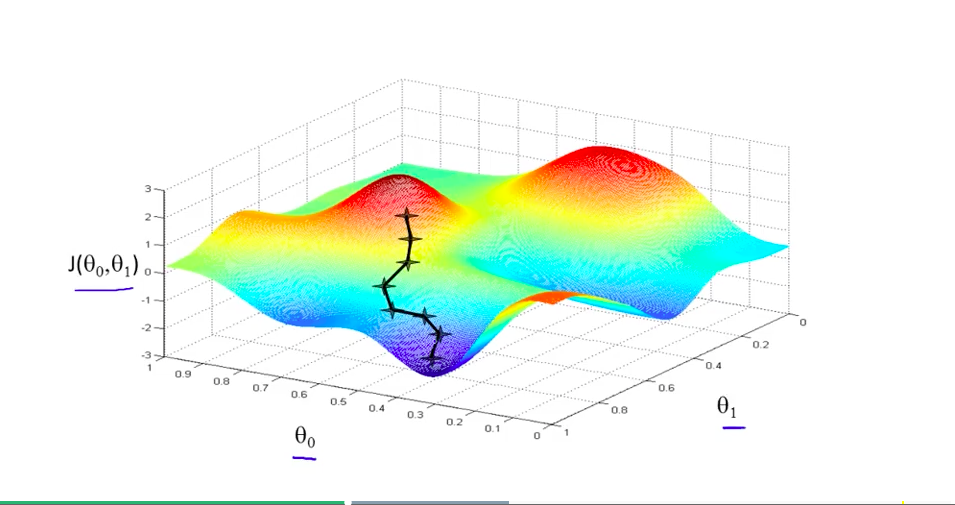
To explain the Solver Options below an analogy of climbing a mountain, to reach the peak (top of the mountain) is used. Our goal is to find the exact parameters that will bring us to the peak of the mountain. Our position on the mountain tells us how high we are (the deviation level), and the direction upwards to the top of the mountain peak (the gradient or mountain slope).
Mountain Climbing with Steepest Decent#
Maximum Number of Iterations#
Value type: integer
This option does not directly control the number of evaluations the solver may run, but instead controls how many attempts the solver will try before giving up.
If the solver attempts to solve more than the maximum iterations the solve will stop.
Tau - Initial Damping Factor#
Value type: float
The tau factor determines whether the solver will try to refine the current parameters a lot (large tau number), or only a small amount (small tau number). Values usually range between +0.0 and +1.0.
Larger values should be used when the initial unknown parameters have high error. This forces the Levenberg-Marquet algorithm to use steepest-decent, rather than gauss-newton.
“The algorithm is not very sensitive to the choice of ‘tau’, but as a rule of thumb, one should use a small value, eg ‘tau = 10-6’, if ‘the initial parameters’ are believed to be a good approximation to the ‘final parameter values’. Otherwise, use ‘tau = 10-3’ or even ‘tau = 1.0’.”
Delta - Amount to Change Parameters#
Value type: float
Delta is the amount of change to the guessed parameters at each iteration.
Each time the solver guesses an unknown parameter value, it adds or subtracts the ‘delta’ value from the unknown parameter value. This changes the magnitude of the parameter values in each guess. If this value is too small, the change in error level may not be detected, if this value is too large the solver will over-estimate and will likely lead to poor convergence (the solver won’t find a good solution).
Epsilon #1 - Acceptable Gradient Change#
Value type: float
The gradient error (sometimes named epsilon #1) is used to find when the solver has reached the “top of the mountain peak”. The gradient represents the slope of climbing the mountain. When the solver reaches a (horizontally) flat area of the mountain, then the gradient is low, and will stop the solve. When the solver can find a slope (gradient), then the solver can follow the slope of the mountain and reach the top of the mountain peak.
At the beginning of a solver iteration, if the solver has not decreased the gradient by at least this value, the solver gives up trying to reduce the error any more, and stops solving.
Epsilon #2 - Acceptable Parameter Change#
Value type: float
The parameter error (sometimes named epsilon #2) is used to determine the when the solver can stop changing parameter values because the new parameter values have not changed enough. Changes to parameters are able to move the solved solution to different places on the mountain, if the parameter changes are too small then the solver will stop.
At the beginning of a solver iteration, if the guessed parameters do not change by at least this value, the solver gives up trying to reduce the error any more.
Epsilon #3 - Acceptable Deviation Error#
Value type: float
The deviation error (sometimes named epsilon #3 or deviation) is the error level that is considered a good solve. To use a mountain climbing analogy, the deviation error is the highest mountain peak that is good enough for the solver.
At the beginning of a solver iteration, if the error level is below this value, the solver considers the error to be low enough for the user’s needs and stops trying to reduce the error.
Auto-Differencing Type#
Value type: integer
The strategy used to compute the direction (gradient slope) the solver should move toward.
Index |
Name |
Description |
|---|---|---|
0 |
|
Fast but not accurate. |
1 |
|
More accurate but 1/3rd slower to compute initially. |
In practice, the authors of mmSolver have found central
dramatically slows down the solver and does not increase accuracy very
much. It is therefore recommended to use forward.
General Solving Concepts#
To be written
Over-Parameterization#
Parameters-errors ratio is too high.
To be written
Plane, Line and Curve Constraints#
To be written
Frequently Asked Questions (FAQ)#
Below are the some common questions and answers.
How do I get the list of supported Solver Types?#
To dynamically get the supported list of solver types, run this Python command in Maya:
>>> maya.cmds.loadPlugin('mmSolver')
>>> maya.cmds.mmSolverType(query=True, list=True)
[u'1=cminpack_lmdif', u'2=cminpack_lmder']   # Example output.
The full list of solver types supported are listed below. Please note that depending on compilation, some solver types will not be available.
What transform space is used for solving?#
MM Solver evaluates all Marker and Bundle screen-space errors in world-space, but solving is not performed in a transform space. Solving is performed directly on Attribute values.
How can I use a DAG hierarchy to reduce the number of Attributes?#
To be written
How can I make my solves faster?#
To be written